Reaction Rates and Rate Laws
Sample page, not class material. It was written to show what a lesson looks like before the class reached Chapter 14, so it may not match how your teacher covers it. Use it as a preview at most.
Practice: Start all 6 questions from Chapter 14 · Pick your own set
On this page 4 sections
Kinetics asks how fast a reaction happens, not how far it goes. This lesson covers three connected ideas: how to write a rate, how a rate depends on concentration (the rate law), and how concentration changes over time (integrated rate laws).
1. Writing a reaction rate
A rate is a change in concentration per unit time. Different species in the same reaction change at different speeds, so we divide by each coefficient to get one rate for the reaction. For the formation of water,
2 H₂ + O₂ → 2 H₂O rate = −1/2(Δ[H₂])/Δt = −(Δ[O₂])/Δt = +1/2(Δ[H₂O])/ΔtSo if O₂ is used up at 0.020 M/s, then H₂ is used up at 0.040 M/s and H₂O forms at 0.040 M/s.
2. Rate laws
A rate law shows how the rate depends on reactant concentrations:
rate = k[A]^m[B]ⁿHere k is the rate constant (it changes with temperature, not with concentration), and m and n are the orders with respect to A and B. The overall order is m + n.
Method of initial rates
Run the reaction several times, change one starting concentration at a time, and compare the initial rates. If doubling [A] multiplies the rate by 2^m, the order in A is m:
| Rate change when [A] doubles | Order in A |
|---|---|
| No change (× 1) | 0 |
| Doubles (× 2) | 1 |
| Quadruples (× 4) | 2 |
The units of k depend on the overall order: M s⁻¹ for zero order, s⁻¹ for first order, and M⁻¹ s⁻¹ for second order. The units are always whatever makes the rate come out in M s⁻¹.
Worked example: find the rate law
For A + B → products:
| Trial | [A] (M) | [B] (M) | Initial rate (M/s) |
|---|---|---|---|
| 1 | 0.050 | 0.050 | 3.0 × 10⁻⁴ |
| 2 | 0.100 | 0.050 | 6.0 × 10⁻⁴ |
| 3 | 0.050 | 0.150 | 2.7 × 10⁻³ |
- Trials 1 → 2: [A] doubles and the rate doubles, so the reaction is first order in A.
- Trials 1 → 3: [B] triples and the rate goes up by 2.7 × 10⁻³/3.0 × 10⁻⁴ = 9 = 3², so it is second order in B.
Rate law: rate = k[A][B]², third order overall.
From trial 1: k = (3.0 × 10⁻⁴)/((0.050)(0.050)²) = 2.4 M⁻² s⁻¹.
3. Concentration over time
Integrated rate laws connect concentration to time. Each one is a straight-line equation, so the order can be identified by finding which plot is linear:
| Order | Integrated rate law | Linear plot | Slope |
|---|---|---|---|
| 0 | [A]_t − [A]₀ = −kt | [A] vs. t | −k |
| 1 | ln[A]_t − ln[A]₀ = −kt | ln[A] vs. t | −k |
| 2 | 1/([A]_t) − 1/([A]₀) = kt | 1/[A] vs. t | +k |
Half-life of a first-order reaction
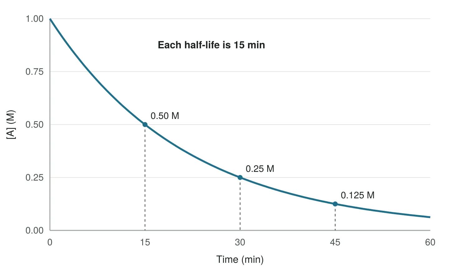
For a first-order reaction the half-life does not depend on concentration:
t_(1/2) = (ln2)/k = 0.693/kThe graph below shows a first-order reaction starting at 1.00 M. Every 15 minutes, half of whatever is left reacts.
Worked example: use the half-life
What is k? k = 0.693/15 min = 0.0462 min⁻¹.
What is [A] after 60 minutes? 60 min is four half-lives, so [A] = 1.00 M × (1/2)⁴ = 0.0625 M.
Check with the integrated rate law: ln[A]_t = ln(1.00) − (0.0462)(60) = −2.77, and e^(−2.77) = 0.0625 M.
Radioactive decay is a common real example of first-order kinetics, which is why half-lives are quoted for isotopes.
Video
This video works through initial-rate problems and integrated rate laws.